From Largecaps to Microcaps: Stock Herding within ETFs

Even before the Flash Crash on May 6, investors and reporters pondered whether ETFs were raising correlations among stocks. Solely buying or selling ETFs directly does not promote correlation. Instead, differences between the ETF's traded price and the indicative net asset value (INAV) create arbitrage opportunities. That difference in price encourages highly efficient traders ("arbitrageurs") to transact in a large sample of stocks underlying the ETF, either buying or selling the stocks and executing an opposing trade in the ETF. Creation Units and Redemption Units further increase the means of executing such arbitrage strategies.

However, arbitrageurs do perform a very important market function for ETFs: they keep the differences between the ETF traded price and the INAV very small (also known to many as "tracking error"). (A very similar term, "basis risk", is commonly used in the context of derivatives, but Fundometry does not seek to blur the lines between ETFs with derivatives any further.) As a result, an ETF will trade closer to its INAV. Or does the INAV trade closer to its ETF? Arbitrageurs likely do not assess which price (ETF or INAV) reflects the true value of a portfolio of equities, but one can argue at length about whether either price reflects fundamental value or the efficient processing of information.

Instead of focusing on how arbitrageurs make a living, this analysis seeks to slice broad equity sectors, according to each stock's market cap, and observe how stocks correlate to their respective ETFs. Frequently, the S&P 500 is cited as the worthwhile benchmark because its components comprise such a large share of the market's value. However, the herding effect of stocks within an ETF may be more acute among for a smaller company, which does not have much analyst coverage to influence its traded price and where less liquidity can create artificial volatility.

The methodology generating the following results is straight-forward. Four ETFs are selected based on their coverage of different segments of the market based on equity market cap.

iShares S&P 500 Index Fund (IVV)
iShares S&P Midcap 400 Index Fund (IJH)
iShares S&P SmallCap 600 Index Fund (IJR)
iShares Russell Microcap Index Fund (IWC) (holding approx 1300-1400 stocks)

The stocks held by each ETF are monitored on a monthly basis, starting with the first quarter of 2008 (an arbitrary point in time but one which avoids too much data squeezing into one graph). Each month, every stock is classified into a quintile based on its weight in the respective ETF. (This assumes that each stock is a member of only one of the four selected ETFs at any one time.) For example, the 100 stocks with the smallest weights in the S&P 500 Index (hence, the smallest 100 stocks by market cap among the 500 largecap stocks) get classified in the lowest quintile ("quintile 1"). By another example, the 120 stocks with the largest weights in the S&P SmallCap 600 Index (the largest 120 stocks by market cap among the 600 smallcap stocks) get classified in the highest quintile ("quintile 5").

Using daily total returns over a 20-day period, a model computes historical correlations between each stock and its corresponding ETF. These correlations are further classified into segments, identified in the graphs below. These segments help to visually demonstrate the breadth of correlation among stocks inside an ETF. If all of these individual correlations were averaged, an important dimension of the outcome would be missing.Finally, these monthly correlations are aggregated into quarterly periods and presented in the following graphs.

The first graph shows the historical correlations among largecap stocks in the S&P 500 index. (Click on any graph to enlarge.)



Above each stacked bar is a quintile number (1 through 5) at the top of the graph, and a legend provides a definition for each numbered quintile. In the case of the S&P 500 index, each quintile contains 100 largecap stocks. Each vertical stacked bar represents the range of correlations for the 100 stocks, as observed during a quarterly period. Represented by different shades of grey, the correlations are grouped according to where they fall within the distribution. Given the wide variations in correlation, among different stocks and over time, the stacked bars provide a more meaningful picture than a simple average or median. (In case median is easier to follow, a red dot depicts the median correlation for each group.)

More often than not, the smallest 100 stocks (quintile 1) within the S&P 500 index correlate more tightly (as viewed by the full height of the stacked bars) than do the largest 100 stocks (quintile 5). As one moves from left to right, the range of correlation broadens in many of the quarterly periods. As one would expect, the overall tightest ranges of correlations occured in 2008Q4, 2009Q1, and 2010Q2, each characteristic of elevated market volatility. Within each quarter, the median correlations (red dots) did not vary materially from the smallest to the largest quintile.

Why might larger stocks within the S&P 500 index have a broader range of correlation than their smaller peers? Liquidity should be fairly deep for all of these largecap stocks. All of these stocks should have reasonable analyst coverage, although larger stocks probably attract more interest from reporters and analysts. Does the availability of more information cause investors to trade a company according to its specific economic fundamentals, as opposed to a less-publicized company being considered part of another largecap basket trade?

Moving down the market cap spectrum, the next graph displays the same correlation profile for the S&P MidCap 400 index.



When looking at the range of correlations within each stacked bar, differences between the smallest and largest quintiles (of 80 stocks) begin to blur over time. In 2008Q1 and 2008Q3, the smallest quintile exhibited the tightest range of correlations among the five quintiles. In some quarters, the largest quintile exhibited the largest range of correlations. As with the largecap profile, the median correlations did not vary materially from the smallest to the largest quintile in each quarter.

The next segment of the market cap spectrum, smallcap stocks, is represented by the S&P SmallCap 600 index.



In this case, the median correlations (red dots) in most quarters showed a steady increase from the smallest quintile (of 120 stocks) and incrementally with each quintile of larger stocks. This pattern is a distinct divergence from the correlation profiles of largecap and midcap stocks above. In certain quarters (2008Q1, 2008Q4, 2009Q4, 2010Q1, 2010Q3), the range of correlations for quintile 1 was materially larger than for other quintiles within the same quarter. As seen from this graph, as smallcap companies moved up in the market cap ranks, their stock prices became more correlated to the S&P SmallCap 600 index.

Finally, rounding out the smallest end of the market cap spectrum is the Russell Microcap Index. (iShares did not license a microcap index from S&P.)



The pattern of increasing correlation with increasing relative market cap was even more prevalent among microcap stocks than smallcap or larger peers. In every quarter, the correlation of stocks to the index (whether based on the median or full range from 5th to 95th percentile) increased as the market cap of the stock increased relative to peers. Quintile 1 exhibited the lowest correlation to the index, in terms of the median and the top/bottom (95th and 5th percentiles) of the stacked bars. Quintile 2 exhibited higher correlations than quintile 1, in terms of the median and 95th and 5th percentiles. This pattern continued through quintile 5 and was remarkably consistent throughout every quarter in the sampled period.

Given the different correlation profiles within each ETF, a convenient summary of these results shows the correlation ranges across the market cap spectrum.



In this final graph, we observe that the median correlation (red dots) increased from the smallest quintile of microcap stocks (quintile 1 of the Russell Microcap Index) to the largest smallcap stocks (quintiles 4 and 5 of the S&P SmallCapp 600 Index). Thereafter, midcap and largecap stocks did not correlate significantly more or less with their respective ETF as their market caps increased. What makes micocap and smallcap stocks different from their larger peers?

1. Mathematically, a cap-weighted index and its corresponding ETF should corrrelate to a greater extent with larger companies in the index or portfolio than with smaller companies. The larger the weight of a specific stock, the greater its influence on the returns of the ETF, hence a higher expected correlation with the ETF over time. The correlation profiles of the microcap and smallcap ETFs were consistent with this premise, but not so for the midcap and largecap ETFs.

2. Despite explanation #1, midcap and largecap stocks of varying weights (quintiles) correlated with the ETF, and plausibly with each other, inside a relatively tight range. Overall, midcap quintile 1 stocks and largecap quintile 3 stocks exhibited the narrowest correlation range among their respective peers. Do arbitrageurs have greater influence on the price movements of the smaller quintile stocks, while a larger population of traders contribute to price movements in the larger quintile stocks?

3. Analyst coverage tends to decline as the market cap of a company declines. Therefore, institutional portfolio managers, and even individual investors, need to spend a greater amount of resources and cost to analyze and monitor smaller companies. Therefore, most investors who gravitate toward investing in largecap stocks can utilize analyst reports and press releases to make trading decisions, which implies a notable factor of company-specific criteria influencing price movements. Conversely, microcap and smallcap investors must invest in more companies (a large "basket" of stocks) in order to diversify their risk to any one company which may suddenly go out of business. In fact, one of the greatest appeals of a microcap ETF is the ability to gain diversified exposure to a market segment which would be otherwise quite expensive to trade (i.e. paying bid-offer spreads and commissions across a very large number of stocks).

4. Microcap and smallcap stocks typically have less liquidity (trading volume) than their larger peers. In order for arbitrageurs to profit from small discrepancies between an ETF and its underlying stocks, transaction costs, specifically bid-offer spreads, must be minimized. Trading a certain numbers of shares within a target bid-offer spread is easier with stocks which have greater trading volumes. Therefore, midcap and largecap stocks should be more favored by traders seeking arbitrage profits between the ETF and its underlying stocks. Microcap and small cap stocks (especially quintiles 1 and 2) would not be liquid enough for such traders. (Also see comment below.)

In fact, a fair absence of arbitrageurs in microcap stocks may explain the steady increase in correlation when moving from quintile 1 to quintile 5. The microcap ETF may provide the best example of how stocks should correlate to an ETF when arbitrage trades are difficult to execute in great frequency, and consequently less profitable. If the microcap segment is the least susceptible to arbitrage trades across a large number of stocks, then it should be the most favorable market segment for traditional fundamental analysts to generate alpha.

Regardless of which explanation, or combination thereof, is the most convincing, stock correlations with an ETF can change significantly depending on company-specific market cap (proxied by weight quintiles) and overall market volatility (proxied by time). One should note that the stocks within a quintile varies from month to month, as their ETF weights change regularly. At the individual stock level, correlations vary substantially from month to month, depending on company-specific news and events. For investors, the more stocks held in a portfolio, the more relevant these results become. For active investors, generating alpha (i.e. outperforming the index) should be more difficult with largecap stocks than with microcap stocks, all else being equal.

From the perspective of public companies, these results probably quantify what CEOs and CFOs already knew. As market cap grows, the more a stock's price becomes influenced by programmatic trading systems supporting index-linked investment vehicles (mutual funds, ETFs, insurance subaccounts, hedge funds, etc). However, at some point, trading volume for a stock may become large enough to dilute the impact of these programmatic factors and increase the influence of analyst coverage and company-specific fundamentals.

This analysis does not dig deep enough to determine how high-frequency trading firms, ETF authorized participants and market structure play a role in the relationship between stocks and their associated ETFs. Hence, the question still remains: "Do ETFs track their INAVs, or is it the other way around?"

Further reading:

The Herd Instinct Takes Over Component Stocks' Correlation to S&P 500 at Highest Level Since '87 Crash (WSJ)

Should ETFs be allowed to include illiquid stocks? (Felix Salmon)

The Real Trend In Fund Flows Will Crush Mutual Fund Managers, And Forever Change The Way Stocks Behave (Clusterstock)

Did nobody ever consider that indexing was dangerous? (FT Alphaville)

Redemptions are Kind to Tax Efficiency, Vanguard ETF Edition

Tax-deferral synergies from bringing together mutual fund and ETF investors

ETF providers promote many benefits of their products: convenience, liquidity, and tax-efficiency, among others. This analysis focuses on some of the mechanics behind tax efficiency, and a unique twist which Vanguard brings to the table with their ETF structure.

Of course, tax efficiency matters when an investor is subject to capital gains taxes. Investors in ETFs can realize capital gains and losses in multiple ways. Buying and selling on the exchanges triggers taxable gains and losses. Like mutual funds, ETFs must distribute any net capital gains realized at the end of the their fiscal year. For a small subset of investors, an in-kind redemption, where an investor exchanges ETF shares for a proportionate number of shares in every stock the ETF holds, can lead to a taxable event for the investor ... but not for the ETF. (Hereafter, we will focus on equity ETFs, not fixed income, commodity, or swap-based ETNs.)

Tax-efficiency can be maximized as long as investors continue purchasing an ETF in sufficient volumes (by way of creation units) while redemptions do not spike for a prolonged period. ETF managers strive to reduce capital gains distributions by trading underlying securities in a manner which offsets realized capital gains with capital losses. The mechanics are no different than with any individual taxable account, in which one tries to harvest losses at opportune times. Ideally, within its underlying securities, an ETF would continue realizing and rolling over net capital losses which can offset any future capital gains.

For Vanguard, the scope of tax-efficiency goes beyond the ETF. Among those Vanguard funds which offer an ETF, the ETF investors and mutual fund investors belong to the same fund. Every investor owns a pro rata share of the same basket of stocks, including all of the associated tax lots. The difference in ownership is signified by the share class. An excerpt from a Vanguard brochure nicely summarizes the benefit to ETF investors:

The more tax lots available, the better a portfolio manager can minimize taxable distributions to all shareholders. This rule applies regardless of whether a fund is a traditional mutual fund or ETF. Thus, when structuring their funds, Vanguard decided to combine the strengths of both the mutual fund and the ETF to maximize tax efficiency.

A historical comparison of two leading Vanguard index funds demonstrates the impact of having mutual fund and ETF investors share the same underlying portfolio. On May 24, 2000, Vanguard launched the ETF share class for the Vanguard Total Stock Market Index Fund. At the time, Vanguard's 500 Index Fund was larger and had existed for a much longer time. However, the ETF share class did not get launched until over ten years later, on September 7, 2010. Did the "patented share-class system" give the Total Stock Market Index Fund advantages which the 500 Index Fund may only be starting to realize?

The annual and semi-annual financial reports for the Vanguard funds provide some very useful details on potential capital gains tax liabilities and the impact of in-kind redemptions ("IKRs"). The following data points, collected from the financial reports, were utilized in this analysis:

1. Realized Net Capital Gains and Losses on securities
2. Realized Net Capital Gains and Losses resulting from in-kind redemptions
3. Purchases and Redemptions by share class.
4. Cumulative Paid-In Capital

Items 1 and 2 directly pertain to the potential capital gains tax liability. Item 3 will help demonstrate the relationship between IKRs and all institutional-size redemptions. Finally, item 4 has a less clear impact, if any, on the potential capital gains tax liability of a mutual fund or ETF. The following excerpt from the latest Vanguard 500 Index Fund semi-annual report helps to explain the relevance of paid-in capital:

During the six months ended June 30, 2010, the fund realized $131,817,000 of net capital gains resulting from in-kind redemptions—in which shareholders exchanged fund shares for securities held by the fund rather than for cash. Because such gains are not taxable to the fund, and are not distributed to shareholders, they have been reclassified from accumulated net realized losses to paid-in capital.

This disclosure is quite common for Vanguard ETFs, as well as ETFs from other sponsors. In fact, Vanguard's index funds disclosed capital gains realized from IKRs even before the ETF class existed. Such disclosures clearly show how good a job the sponsor does at removing share lots of underlying securities with the largest capital gains (without incurring any immediate tax liability). When capital gains are realized from IKRs, the fund simply reclassifies them as paid-in capital. (More specifically, these capital gains are added to paid-in capital instead of increasing Accumulated Net Realized Gains or offsetting Accumulated Net Realized Losses.)

In terms of tax efficiency, how has the tax profile of the 500 Index Fund fared over the last ten years? The following graph shows the two sources of paid-in capital — new investments (green bars) and capital gains resulting from IKRs (yellow bars) — and compares them to the taxable realized capital losses (red bars).

As the fund AUM grows over time due to new investments (rising green bars), so does the cumulative balance of IKR capital gains classified as paid-in capital (yellow bars). In fact, those capital gains resulting from IKRs are almost as large as the accumulated net realized capital losses (red bars). If the yellow bars did not exist, how would the tax profile haved fared over the same period?

For tax years 2001 and 2009, the 500 Index Fund would have been forced to make capital gain distributions to all classes of shareholders, proportionate to the value of shares allocated to each class and shareholder. The tax-deferral benefit from IKRs (presumably from institutional investors who have positions large enough to warrant accepting the underlying 500 securities instead of cash) accrues to all classes of shareholders.

We can assume that retail investors accessed this fund through the Investors share class. The other classes (Admiral and Signal) have lower expense ratios but much higher minimum account size requirements, hence more appropriate for institutional investors. How does the redemption activity of institutional investors compare to that of individual investors?

In most years, the value of institutional shares redeemed for cash or in-kind (red bars) is a fraction of the equivalent amount for retail shares (green bars). Furthermore, the capital gains classified as paid-in capital represent an even smaller fraction of these redemptions.

The following graphs convey the same data for the Total Stock Market ("TSM") Index Fund, which launched its ETF share class on May 24, 2000. (Remember, the 500 Index Fund did not have an ETF share class until after its latest published financial report.)

First, the AUM growth rate for the TSM Index Fund (depicted by the increasing green bars over time) is much higher than that of the 500 Index Fund. Normally, such a large and consistent inflow of new investments would give the portfolio manager ample flexibility to minimize capital gain distributions to shareholders. In fact, the magnitude of tax-deferral is impressive as the portfolio manager realized only net capital losses (red bars) since 2000. These capital losses are more than offset by the paid-in capital resulting from IKRs (yellow bars).

However, excluding the impact of IKRs, the tax profile changes significantly.

In every tax year, the fund likely would have made capital gain distributions to shareholders. Thanks to IKRs, the portfolio manager was able to avoid a series of capital gain distributions and retain more AUM (from which the manager's fees are computed).

The following graph shows historical redemption activity for retail and institutional investors. For the TSM Index Fund, institutional investors are deemed to have utilized the Institutional and ETF share classes, both of which do not exist in the 500 Index Fund. The Vanguard Institutional Index Fund, which also holds approximately 500 stocks, offers institutional share classes, but its financial and tax books are entirely separate from those of the 500 Index Fund. Perhaps differences in legal opinion explain the separation.

Here one can observe that the amount of capital gains resulting from IKRs (yellow bars) fluctuates consistently with the amount of institutional and ETF shares redeemed (red bars). (ETF redemptions are presumed to always be in-kind redemptions since the other means of liquidating an ETF position — via the seconday market — is not a redemption from the fund's perspective.) As long as IKRs keep occurring, the portfolio manager should be able to continue realizing net capital losses every tax year. Of course, if the market rallies strongly and steadily, the manager may run out of tax lots with embedded capital losses. (One could think of worse challenges to have.)

On the surface, everyone appears to have benefitted. The portfolio manager removes the largest capital gain tax lots from the fund, reducing the likelihood of realizing net capital gains in future tax years. If the fund continues to realize only net capital losses every tax year, a capital gain distribution should not occur, thus avoiding a taxable event for investors in non-qualified accounts. However, by avoiding a capital gains distribution, the AUM of the fund does not decrease either, increasing the management fee incrementally. Only when an investor eventually sells shares, either back to the mutual fund or in the ETF's secondary market, a capital gains tax liability could be incurred. Essentially, those net capital gains resulting from IKRs, including any unrealized net capital gains, are accumulated within the fund's NAV and become taxable when an investor redeems shares. Whether the capital gains are classified as long-term or short-term depends on the holding period of the fund investor, not the fund's holding period at the underlying security level.

Long-term investors benefit the most. Not only do they avoid receiving taxable distributions until redeeming fund shares, their profits should be mostly (or entirely, depending on investor-specific holding periods) taxed at the lower long-term capital gains tax rate. Short-term investors should benefit, but not necessarily in all cases. If a short-term investor (who holds a position under one year) realizes a capital gain, the entire gain would presumeably be taxed as current income (subject to the investor's specific circumstances, of course). If instead the investor had received a capital gain distribution from the fund (which likely could have happened if not for the IKRs), part of the distribution may have been classified as long-term capital gains (pursuant to the portfolio manager's choice of which security-level tax lots to sell). Since Vanguard promotes long-term investment horizons, one can understand the focus on benefitting long-term investors.

This brief analysis does not draw any new conclusions. Rather, the comparison between two leading Vanguard funds, one with and one without an ETF class, demonstrates the importance of in-kind redemptions on tax efficiency. Investors in the Vanguard 500 Index Fund should look forward to greater tax efficiency in the future. What about the investors in the Vanguard Institutional Index Fund, which does not offer an ETF class? Could a very large fund merger be on the horizon?

ETF Trade Execution Quality during the Flash Crash Month

Subtitle: Some market orders received better price execution than limit orders.

Recently, all market centers disclosed Rule 605 reports for May 2010. This data provides insights into the quality of trade execution across all market centers by ticker, order size, and order type. The following analysis focuses on a favorite focus point of the Flash Crash debate: ETFs. By utilizing the Rule 605 disclosures for May 2010, a volatile month for equities trading, we can observe where ETF trades received better price execution.

There are no clear strong or weak points apparent in the numerous graphs below. Each reader may have an interest in specific ETFs or market centers. Unfortunately, there are too many permutations of ETFs and market centers to be covered within this post. The following graphs sample a few ETF complexes and market centers with the highest trading volumes during May 2010.

More importantly, Rule 605 disclosures summarize trades for the entire month, not itemized by day. Hence, the following graphs do not solely represent trading activity on May 6, 2010, when many ETF orders were cancelled as a result of extreme price volatility resulting from brief market illiquidity. (Judging from the wide range of price improvement statistics, these cancelled trades appear to be included in the data, but one cannot assume the all market centers included erroneous trades in their disclosures.) For some ETFs and specific market centers, the price volatility on May 6 may have been large enough to significantly impact the summary statistics for the entire month. Nevertheless, a comparison of the same statistics across ETFs and market centers should demonstrate how trade execution performed on a relative basis.

In previous posts (iShares/NFS and Schwab/UBS) concerning ETF trade execution quality, Fundometry studied how much trades were executed inside the NBBO, at the market, and outside the NBBO for specific market centers. One post defined a useful summary metric called Weighted Average Price Impact ("WAPI"). In the Rule 605 disclosures, price impact (in dollars per share) is disclosed separately for trades where price improved and degraded (or, as some might say, disimproved) relative to the subsequent NBBO. The overall price impact of trades can be summarized by averaging the price impact for individual categories of trades, based on improvement or degradation relative to the NBBO and weighted according to respective volumes in each category. A positive WAPI indicates that overall more shares traded with price improvement (i.e. price at execution was better than the NBBO when the order was submitted) than with price degradation, and the opposite would be implied by a negative WAPI.

In addition to WAPI, the following graphs plot volume of executed orders, including orders routed to other market centers. Ideally, this data on trade execution would be itemized separately for internal orders and orders routed to other market centers (in cases where the best price existed at another venue). Unfortunately, the data summarizes trade execution quality across all orders executed regardless of venue (internal or external). In order to highlight the impact of orders executed internally to any given market center, only data is included if the volume of internal orders contituted at least 80% of total executed volume. (The final graphs in this post follow a stricter threshold of 5%.)

Finally, both WAPI and volume are broken down by market orders and marketable limit orders - the only two types of orders for which price improvement/degradation statistics are available.

Based on the Rule 605 disclosures sampled in this analysis, three ETF complexes had the largest trading volumes of market and marketable limit orders during May: SPDR, iShares, and ProShares. Initially, ETFs will be summarized at the complex-level (volume-weighted summary of all tickers within an ETF family) across different market centers (exchanges, ECNs, ATS, etc). Subsequently, selected individual ETFs will be analyzed in greater detail, by order size and order type. (Given the number of graphs involved, including other ETF complexes or selecting more individual ETFs would cause this post to become rather voluminous.)

Complex-Level Perspective

In these complex-level graphs, market centers displayed along the horizontal axis are sorted according to overall WAPI. Market centers which executed orders with overall price degradation (outside the NBBO recorded at the time the order was submitted) are displayed closer to the left side. Despite this sorting order, some market centers achieved notably better or worse trade execution quality depending on the order type (market vs marketable limit).

The following graph summarizes trade execution quality for SPDR ETFs during May 2010.

For the SPDR family of ETFs, a few low-volume market centers exhibited the least favorable trade execution quality. Among market centers with notable volume, National Financial Services (NFS), BATS, and Knight Capital Markets performed less favorably relative to their peers, in terms of WAPI. Depending on the market center, market orders received better price execution than marketable limit orders (as seen when red diamonds are higher than blue diamonds). While there is no clear indication of where market orders should have fared better, marketable limit orders (a buy order above the best offer or a sell order below the best bid) did not always result in better price execution than market orders.

The following graph, which summarizes trade execution quality for iShares ETFs during May 2010, shows that orders executed at UBS, Knight, and Chicago Stock Exchange (CHX) Matching System received less favorable price execution relative to their peers. CHX and NFS executed market orders (red diamonds) at better prices than marketable limit orders (blue diamonds), but the opposite was the case at UBS and Knight. Direct Edge X exhibited the most negative WAPI among market orders.

The following graph for ProShares ETFs shows that Knight Equity Markets executed marketable limit orders with a reasonable WAPI but achieved relatively poor execution quality with market orders. Conversely, Knight Capital Markets achieved reasonable WAPI for both types of orders. Among peers, Oppenheimer exhibited the best WAPI for marketable limit orders but performed poorly with market orders. Again, one can observe how order type matters depending on the venue.

Focus: SPDR ETFs

The graphs above summarize trade execution quality for different market centers across all ETFs within a single family. Conversely, the following graph summarizes trade execution for different ETFs in the SPDR complex across all market centers.

Two ETFs with the least favorable WAPI, XSD and XBI, exhibited worse price execution for market orders than for marketable limit orders. Otherwise, market orders received more favorable execution, based on price, than marketable limit orders for most of the other tickers (even though volume for market orders was substantially lower than for marketable limit orders). In comparison to other tickers, MDY and GWX exhibited less favorable price execution for marketable limit orders. These four ETFs merit more detailed analysis.

The following graph drills down into trade execution quality by order type and order size for XSD.

Interestingly, two specific categories of market orders account for the unfavorable WAPI: (1) order quantity 2000-4999 (order size code "C") executed at UBS Securities and (2) order quantity under 500 shares (order size code "A") executed at Knight Capital Markets. Furthermore, the most favorable WAPI for market orders in this graph occurred at Knight Capital Markets for order quantity over 5000 shares (order size code "D"). Given that the fragmentation of market structure generally favors smaller orders for achieving better execution quality, the results at Knight are unexpected.

Does the same graph for XBI result in similar observations?

Yes and no. As was the case for large-quantity market orders for XSD executed at Knight, the largest-quantity market orders (2000-4999 shares) for XBI executed at NYSE Arca achieved the most favorable WAPI, certainly better than smaller-quantity market orders. At Knight, larger market orders (2000-4999 shares) received substantially less favorable WAPI than market orders with the largest-quantity (over 5000 shares). However, at Automated Trading Desk, the largest-quantity market orders (over 5000 shares) received substantially unfavorable WAPI than all other comparable orders on this graph. (Note that the total volume on some of these categories of market orders is very small.)

In the two graphs above, the WAPI for marketable limit orders was very consistent relative to market orders. Two SPDR ETFs which exhibited unfavorable execution, based on WAPI, for marketable limit orders are MDY and GWX. The following graph drills down into trade execution quality for MDY.

Marketable limit orders for MDY executed at Barclays Capital and Direct Edge X received increasingly less favorable WAPI as the order size increased. This pattern follows the broad expectation that smaller orders receive better price execution. To a lesser extent, the same pattern is evident at BATS Exchange and NASDAQ. However, market orders received more favorable WAPI than marketable limit orders, based on comparable order sizes.

The same graph for GWX yields less conclusive observations.

At NYSE Arca, Knight Capital Markets, and UBS Securities, marketable limit orders received better WAPI when the order size was smaller, but the opposite trend occurred at LavaFlow ECN (where volume was also lower). At UBS Securities, market orders received better WAPI when their order size was smaller, but at Knight there was no conclusive pattern to how well a market order would be executed according to its size.

Focus: iShares ETFs

Switching from the SPDR to iShares complex, the following graph summarizes trade execution for different ETFs in the iShares complex across all market centers.

Two ETFs stand out in terms of unfavorable WAPI for market orders: IWV and IWR. In addition, for marketable limit orders, EFG exhibited a less favorable WAPI than its peers. The following three graphs analyze what happened with each of these iShares ETFs.

For IWV, one could easily miss any anomalies in the trade execution quality. The red diamond at the lower left region represents substantially negative WAPI for large-quantity market orders executed at Knight Capital Markets. Smaller market orders at Knight received better execution. Other market centers exhibited reasonable results.

The results for IWR are surprisingly consistent with IWV. Large-quantity market orders executed at Knight received substantially negative WAPI, as indicated by the red diamond in the lower left region. The remaining data points are easier to view when this one negative outlier is excluded from the graph.

Across all five market centers, marketable limit orders received less favorable WAPI as the order size increased, with a few exceptions. At Knight, only the smallest-quantity market and marketable limit orders achieved positive WAPI. At NYSE Arca, market orders once again exhibited more favorable WAPI than marketable limit orders of comparable order size. While Automated Trading Desk executed market orders with more favorable WAPI as the order size decreased, the same pattern could not be observed for marketable limit orders.

Before switching focus to EFG, one may wonder whether orders for other iShares ETFs exhibited substantially negative WAPI at Knight. The following graph indicates that IWV and IWR were unique outliers, but some other ETFs also exhibited less favorable WAPI for market orders: IVW, IWP, IJT, IJH, and IJR.

For EFG, the least favorable WAPI for marketable limit orders occurred at E*Trade Capital Markets, although the magnitude is insignificant when compared to results for IWV and IWR.

At E*Trade, the largest-quantity marketable limit orders for EFG exhibited substantially unfavorable WAPI versus other market centers. Knight Capital Markets executed marketable limit orders with improving WAPI as the order size increased (again, counter to expectations based on general market structure). Even NYSE Arca and Pershing followed a similar pattern with respect to market orders (i.e. more favorable WAPI as order size increased), except when Pershing executed the largest-quantity market orders.

Focus: ProShares ETFs

The following graph summarizes trade execution for different ETFs in the ProShares complex across all market centers.

As shown in the next two graphs, both SQQQ and UPRO exhibited similar patterns to earlier examples for selected SPDR and iShares ETFs. In the case of SQQQ, market orders of quantity 2000-4999 executed at Knight Capital Markets received the least favorable WAPI, although not of significant magnitude in comparison to IWV and IWR.

For UPRO, the largest market orders executed at Knight received the most negative WAPI.

However, for ROM, market orders of the largest-quantity (5000 or more shares) exhibited the least favorable WAPI at Citadel Securities, although Knight and Automated Trading Desk also executed market orders with relatively less favorable WAPI.

Conclusions

Depending on the market center and specific ticker, trade execution quality, as measured by Weighted Average Price Improvement, varies wildly. As seen in the graphs above, robust generalizations are difficult to draw.

1. Marketable limit orders do not always receive better price improvement than market orders. Marketable limit orders are limit orders which should be executed immediately, as with market orders, because either the order bid is higher than the best offer or the order offer is lower than the best bid. Depending on the market center, market orders can receive better price improvement versus marketable limit orders of comparable order size. In other words, executing a market order may result in price improvement despite the fact that many erroneous trades involved stop loss market orders.

2. Depending on the specific ETF, market center does matter. Among the small sample of graphs above, some market centers repeatedly achieved less favorable price improvement than their peers. The Rule 605 disclosures cover only orders for which a market center was not specified by the investor. As a result, the data should reflect efforts to route orders to the market center which has the best NBBO at a given time. However, identifying the reasons why an order executes at a specific venue requires more data than available through the Rule 605 disclosures.

3. Major market centers with a large share of volume (usually synonymous with deep liquidity) do not necessarily achieve better price improvement. Regardless of trading volume, some market centers appear to execute market orders with better price improvement than for marketable limit orders. The same complex-level graphs shown above are available with market centers sorted from left to right in order of trading volume: SPDR, iShares, ProShares.

4. Typically, order size does matter. Depending on the market center and individual ETF, smaller orders might achieve better price improvement than larger orders, but many instances of the opposite exist. At least one should not assume that smaller orders always achieve better price improvement, especially with market orders. Since some trade execution statistics are based on small order volumes, one should study more periods of history in order to draw statistically robust conclusions.

For those seeking a more league-tablesque summary, the following graphs may be more satisfying. These graphs list the most and least favorable price improvement performances for combinations of individual ETFs and market centers. Market orders and marketable limit orders are shown separately, as their overall magnitudes of WAPI are different.

One of the market centers should be familiar by now (if not, this WSJ article might help). For those seeking a comparison, the same graphs for April are available for market orders and marketable limit orders.

Clearly, May was an exceptional month as highlighted by the price impact of ETF trades. In such challenging and volatile markets, is the quest for price improvement worthwhile, or would a market center be better off routing an order elsewhere? For investors, the dilemma is even more complicated: which ETF, order type, and order quantity would work best? There can be no assurance that if Flash Crash II ever occurs, the quality of price improvement will follow similar patterns.

Using Leveraged ETFs to Trade during Circuit Breakers

Subtitle: Intraday Correlations between ProShares ETFs and Broad Market Indices

On June 30, 2010, the SEC announced its intention to expand the circuit breaker pilot program to many more stocks and, for the first time, ETFs. Public comments have expressed concern that, when applied to ETFs, circuit breakers may themselves create market disruptions. If a circuit breaker is triggered, whether appropriately or erroneously, for a widely-traded ETF, HFT firms major market participants may pause trading and deprive the market of liquidity when it is most needed. Once an ETF selected for the pilot program triggers a circuit breaker, firms which trade the basket of underlying stocks may also step away for five minutes until trading in the ETF resumes. In such a scenario, the impact on the liquidity of stocks underlying a halted ETF will demonstrate whether the circuit breaker program meets its objectives in practice.

Not all ETFs have been selected for the circuit breaker pilot program. NYSE Euronext compiled a list of 344 ETFs ("piloted ETFs"), as reported by Index Universe, utilizing a volume cutoff:

"NYSE Euronext, the parent company of the New York Stock Exchange, developed the list of 344 ETFs in consultation with other major exchanges and the Financial Industry Regulatory Authority.

"NYSE Euronext winnowed down the universe of U.S. ETFs by excluding products whose average daily trade volume was less than $2 million worth of shares, it said in a press release."

This criteria for selected ETFs produces some interesting and potential trading scenarios. For example, SPY and IVV, two ETF's which track the S&P 500, are included in the proposed expansion of the circuit breaker program. Therefore, if one of these two ETFs triggers a circuit breaker, will the market simply move to trade the other ETF until five minutes passes? What are the odds that both SPY and IVV will simulateously trigger circuit breakers? (This is not a rhetorical question.)

Given the complex trading relationships between an ETF and its underlying stocks, concerns about market disruption resulting from a circuit breaker are difficult to prove in theory and potentially difficult to quantify. A further review of the list of ETFs proposed for the circuit breaker pilot program reveals another interesting scenario: if a broad-market ETF triggers a circuit breaker, can traders utilize leveraged versions of the ETF to continue trading through the duration of the circuit breaker?

To address that possibility, we start with a summary of ETFs which may serve as substitutes (or proxies) for three broad market ETFs: SPY, QQQQ, and IWM.

Those ETFs participating in the circuit breaker pilot program are only unleveraged (long and short) versions of their underlying indices. The obvious choice for trading through the duration of a circuit breaker would be to use a leveraged (long or short) ETF, sponsored by ProShares. The remainder of this analysis studies how effectively these ProShares ETFs followed their stated leverage ratio during 2010 Q2.

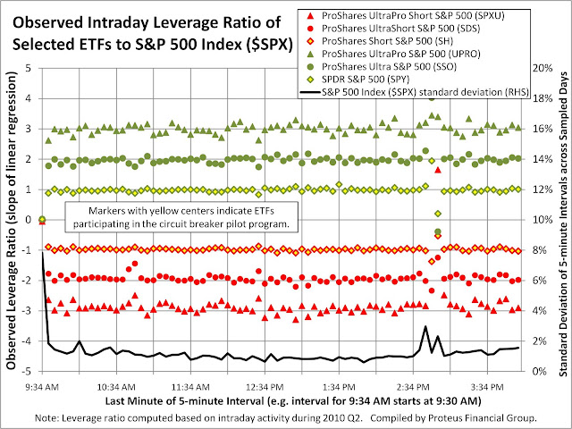
First a definition of the term "leverage ratio" as utilized in this analysis. To take an example, the ProShares Ultra S&P 500 (SSO) has a stated objective of going up or down twice as much as the S&P 500 index, on an intraday basis. Hence, the stated target leverage ratio for SSO is +2. Conversely, the stated target leverage ratio for ProShares UltraShort S&P 500 (SDS) is -2 because SDS moves in the opposite direction to the S&P 500. By looking at the returns of leveraged long/short ETFs over 5-minute intervals during 2010 Q2, we compare their returns to the underlying index by utilizing linear regression analysis. These regressions are constrained to have a zero alpha (zero intercept) so that the resulting beta (slope) provides a useful (albeit not perfect) measure of the leverage ratio. Each regression compares a single ETF to its underlying index, ignoring any 5-minute intervals when such ETF did not trade. Otherwise, volume has no impact on the regressions. By constraining the alpha to zero, the following graphs need to display only the slope (termed the "observed leverage ratio").

The closer an ETF trades to its stated target leverage ratio, the better such ETF may serve as a proxy if another related ETF triggers a circuit breaker. How well might various leveraged long/short ETFs of the S&P 500 index serve as proxies to SPY, IVV, or SH? The following graph shows the consistency of the leverage ratio for every trading day furing 2010 Q2.

(For convenient viewing throughout all graphs, those ETFs which will be subject to circuit breakers have markers with yellow centers. For graphs pertaining to the S&P 500, the iShares ETF is excluded so that the higher-volume SPDR ETF is easier to view. On graphs plotting the observed leverage ratio over time, a black line represents the daily standard deviation of 5-minute returns to help compare deviations in the observed leverage ratio to underlying index volatility.)

On a daily basis, the leveraged ETFs appear to trade according to their stated target leverage ratios. As the target level rises to 2x and 3x, the observed leverage ratio for both long and short ETFs exhibits greater variability around the target level. Perhaps the efficiency of instruments used to gain leverage suffers as leverage rises. Liquidity might also play a role. Leveraged ETFs typically have lower trading volume than their corresponding long unleveraged ETFs (discussed in detail further below).

Can one draw the same conclusion by looking at the observed leverage ratio over intraday 5-minute intervals? In this graph, the leverage ratio is computed through a linear regression utilizing all trading days during 2010 Q2 but for a specific 5-minute interval during each trading day.

During certain times of the day, on average, the observed leverage ratio tended to deviate from the stated objective. Most likely (especially between 2:30 and 3:00) these deviations reflected aberrant activity on specific days (e.g. May 6), as opposed to repetitive behavior during most trading days. Interestingly, the interval from 9:30 to 9:34, where 5-minute volatility is highest overall, shows the largest discrepancy in observed leverage ratio. Currently, the SEC does not apply circuit breakers during the beginning and end of regular trading hours (9:30 to 9:45 and 3:45 to 4:00).

Switching from a time-based perspective, the next graph shows the observed leverage ratio according to the return in the underlying index during 5-minute intervals.

(For clarification, the horizontal axis shows return bands, each spanning 0.10%. The return band labelled -0.30% includes any 5-minute intervals when the underlying index dropped by 0.3000% to 0.3999%. The return band labelled +0.30% includes any 5-minute intervals when the underlying index rose by 0.2001 % to 0.3000%. The return band labelled 0.00% includes any 5-minute intervals when the underlying index dropped by -0.0999% to 0.0000%. Furthermore, since the return bands are based on the underlying index, and not the ETFs, circuit breakers might have triggered if they had been in effect for ETFs at that time.)

All ETFs based on the S&P 500 traded close to their stated target leverage ratios as long as the underlying index did not rise or fall more than 0.40% within any 5-minute interval. As the underlying index became more volatile, the observed leverage ratio tended to shrink. Note that as the magnitude of change increases, the number of historical data samples drops, which may in turn reduce the regression quality and increase the standard error of the slope (beta).

In the same manner, we can determine how well various leveraged long/short ETFs of the NASDAQ 100 index served as proxies to QQQQ or PSQ. The following two graphs plot the observed leverage ratio over time, first daily followed by intraday, and roughly follow the patterns seen in the graphs for the S&P 500. For the ProShares triple-leveraged ETFs, SQQQ and TQQQ, the observed leverage ratios deviated from the stated target levels more so than for the corresponding ProShares ETFs tracking the S&P 500 .

According to the return in the NASDAQ 100 during 5-minute intervals, the following graph shows that the observed leverage ratios for the related ETFs tracked their stated target levels most of the time. Only when the Nasdaq 100 index rose or fell by more than 0.40% did the observed leverage ratio begin to decline. In this case, the spike in standard error which we observed for the S&P 500 is not present among the ETFs which track the NASDAQ 100.

Finally, we can determine how well various leveraged long/short ETFs of the Russell 2000 index serve as proxies to IWM or RWM. The following two graphs plot the observed leverage ratio over time, first daily followed by intraday.

In this case, the observed leverage ratio of the ETFs fluctuated even more from their stated objective than for the ETFs which track the NASDAQ 100. Could these fluctuations be the result of lower trading volume in the ETF and its component stocks? Additional analysis further below should address this question.

According to the return in the Russell 2000 during 5-minute intervals, the following graph shows that the observed leverage ratios tracked (and many times exceeded) the stated target levels most of the time. Only when the Russell 2000 index rose or fell by more than 0.50% did the observed leverage ratio decline significantly.

Thus far, the leveraged ETFs corresponding to the S&P 500, NASDAQ 100, and Russell 2000 appear to maintain an observed leverage ratio consistent with expectations, except during sharp price movements. However, brief periods of sharp price movements would be most likely to trigger circuit breakers, outside of erroneous trading activity. Might the participation of unleveraged ETFs in the circuit breaker pilot program prompt a change in how leveraged ETFs behave during extreme price volatility? In other words, can leveraged ETFs attract more volume, and in turn achieve observed leverage ratios consistent with stated levels, if any of their corresponding unleveraged ETFs triggers a circuit breaker?

The following three graphs compare the daily volume of the ETFs listed above (except for IVV). When selecting ETFs to include in the pilot program, the SEC focused on the highest-volume ETFs for the three broad-market indices. In addition, the corresponding unleveraged inverse ETFs had respectable volumes but lower than some of their leveraged counterparts. (Note the log scale for the vertical axis.)

In fact, for all three indices, the double-leveraged ETFs (both long and short) traded with materially higher volumes than their corresponding unleveraged short counterparts. The same conclusion can be drawn from the following three graphs, which plot average intraday volume during 5-minute intervals according to the 5-minute return in the underlying index. (Note that the graph plots average, not total, 5-minute volume because not all ETFs traded during every interval in every trading day of 2010 Q2.)

Once again, the double-leveraged ETFs consistently traded in greater volumes than their unleveraged short counterparts but less than their unleveraged long counterparts. Furthermore, these three graphs exhibit a very consistent "smile" shape, indicating that 5-minute interval volume does increase as 5-minute price movement (positive or negative) increases. While the overall shape is intuitive, the consistency among all ETFs (across different leverage ratios and long vs short) demonstrates the potential for a leveraged ETF to attract more volume should an unleveraged long or short ETF trigger a circuit breaker. However, these graphs do not and cannot prove how the observed leverage ratio of leveraged ETFs might behave during such a market scenario in the future.

In conclusion, the above analysis demonstrates some key aspects of leveraged ETFs which require careful consideration during normal and volatile periods of intraday trading.

1. As intraday (5-minute interval) price volatility of an underlying index increases, the observed leverage ratio drops significantly below stated levels. If an underlying index rises or drops by more then 0.50% in a 5-minute interval, then the leveraged ETFs may not trade at a predictable correlation to the undering index within the same interval.

2. As intraday price volatility of an underlying index increases, the corresponding volume also increases, confirming that ETFs are popular among traders who seek to rapidly gain market exposure or hedge existing positions. Both leveraged and unleveraged ETFs exhibit the same pattern of trading volume, which demonstrates that a leveraged ETF may be a viable proxy for an unleveraged ETF which has triggered its circuit breaker.

3. Both the NYSE and SEC appear to have postponed determining how leveraged ETFs may be included in the circuit breaker program. Most likely, the embedded leverage of such ETFs increases their chance of triggering a circuit breaker at times when other similar ETFs may trade inside their trigger levels. Such a potential scenario is further complicated by past behavior of observed leverage ratios, as shown above. (Currently, the SEC is not granting exemptive relief to ETFs which request to make significant investments in derivatives.)

4. The SEC is already concerned with the performance of leveraged ETFs, specifically due to their daily resets (which should not be pertinent to intraday leverage ratios). Might the exercise of identifying circuit breaker trigger levels create further scrutiny on a product where FINRA states "typically are not suitable for retail investors who plan to hold them for more than one trading session, particularly in volatile markets"?

Once the proposed ETFs are rolled out into the circuit breaker pilot program, leveraged ETFs will be put to a potentially new test . How might leveraged ETFs behave empirically should a related ETF trigger its circuit breaker?

Drilling Down into the Flash Crash, ETF Edition

Many media reports have commented on the severity with which stock prices collapsed during the afternoon of May 6, 2010 ("Flash Crash"). The most surprising casualty from the Flash Crash are ETF's. In general, ETF prices fluctuate consistently with the underlying index (for passive indexed, not active, portfolios) due to sufficient trading volume in the ETF itself and/or the ability for authorized dealers to use baskets of the underlying securities to profit from pricing discrepancies between the ETF and its constituent securities. ETF Trends wrote an article (referenced below) discussing the mechanisms for trading large blocks of ETF's either directly or indirectly via its constituent securities.

While ETF's justifiably raised concerns in light of the Flash Crash, the media has portrayed ETF's as a single asset class in this context. Some Wall Street Journal articles (referenced below) have presented examples of specific ETF's which suffered from extreme volatility that day. Although most of the trades which the exchanges cancelled on the evening of May 6 occurred in ETF's, many other ETF's did not incur enough price volatility to require trades to be cancelled. Few, if any, reporters have drilled down to determine which types of ETF's, and their sponsoring firms, performed better or worse on May 6.

This article attempts to reveal important distinctions among US-listed ETF's during the Flash Crash. In order to simplify the analysis, certain ETF's have been excluded. Those ETF's which utilize derivatives to achieve leverage (funds named with "ultra", "2x", "3x", and "double") are excluded in all comparisons because, by definition, their volatility is supposed to be higher than the general market, which would be confused with the exceptional volatility of un-leveraged ETF's on May 6. For similar reasons, inverse ETF's (funds named with "bear" and "short") are excluded. While the market was falling precipitously on May 6, inverse ETF's, by definition, should have not surprised investors in the same manner as long-only ETF's. Studying a single date of performance gives a limited scope of observations, but, nevertheless, readers can draw some very useful conclusions to help make future decisions on how to utilize ETF's in short-term trading or portfolio management strategies.

The simplest way to focus attention on the ETF's which exhibited unusually high volatility is to break down performance according to broad sectors. In the following table, we observe some sectors with severe price declines on May 6 regardless of high or low trading volume. The extreme magnitude of downside volatility is measured by how low prices fell in relation to the closing price that day ("Low-to-Close Difference", or "LCD"). For example, an ETF which traded as low as $1 but closed at $10 on May 6 would have an LCD of 90%. In order to better reflect the overall impact on market participants and investors, each ETF's LCD is weighted by the trading volume on May 6 to arrive at the Weighted Average Low-to-Close Difference ("WA-LCD"). Admittedly, a more accurate weighted average would consider the trading volume during the brief time during which most of the intraday volatility occurred, but that data requires more time to aggregate and process (perhaps a worthwhile objective for a future article on Fundometry).

As expected, ETF's invested in equities, including Asset Allocation, suffered from the most severe price drops. Large Cap (US) Equity ETF's performed better than Mid/Small Cap (US) Equity ETF's, which is consistent with the history of higher observed volatility in the prices of smaller companies. While the Asset Allocation sector exhibited the largest overall drop in price, that performance spans a broad range at the level of specific sectors (Moderate Allocation, Target Date, etc. as seen further below). Perhaps most significant, several sectors should be credited with avoiding the extreme price volatility of May 6: Taxable Bond, Municipal Bond, Global Bond, Currency, and Commodity ETF's. Finally, even though a broad sector may exhibit modest volatility overall, a single ETF within the sector may have performed much more poorly, as evidenced by the rightmost column "Worst Single ETF Low-to-Close Difference".

The next logical step in this analysis is to compare sectors which comprise the above broad sectors. The tiering of performance across specific asset classes and investment styles is quite apparent in the following table.

Clearly, the Small Cap Equity and Mid Cap Equity sectors rank among the worst performing sectors on the basis of the lowest trading price. Among the Small/Mid Cap group, the Small Cap Blend Equity sector held up by and far the best, with a weighted average lowest trading price 7.04% below the weighted average closing price. Industry-specific sectors suffered some excessive volatility, led by Telecom Sector Equity on relatively low volume. In order to judge the relative performance on most sectors, the Large Cap Blend Equity (which includes ETF's tracking the S&P 500) may be the benchmark. Sectors investing overseas performed relatively better. Among fixed income ETF's, the High Yield Bond sector exhibited the most downside volatility, trading 7.00% below the closing price on a weighted average basis. Relative to most sectors, the remaining bond sectors, as well as Commodity, Currency, and Target Date sectors, suffered limited downside volatility during the Flash Crash and exhibited the least negative WA-LCD figures.

Different ETF's sponsors offer products spanning various sectors. Therefore, when drilling further to the sponsoring firm level, the following tables each compare performance within a single broad sector. The term "ETF Complex" includes the ETF's offered by one firm, or within one family, which fall within the specified broad sector, and each WA-LCD is computed accordingly. The first table below compares ETF Complexes which offer Large Cap Equity portfolios.

At the ETF Complex level, trading volume shows a stronger correlation to the WA-LCD metric. ETF's from FaithShares and Grail have the lowest trading volume among their peers, perhaps to the extent that these ETF's did not trade much during the most volatie period on May 6. The leading ETF Complexes by volume - PowerShares and State Street SPDR's - performed consistently with the broader market primarily because of their high-volume products - QQQQ and SPY, respectively. (Remember, WA-LCD is weighted by trading volume on May 6.) The next most-traded ETF Complex - iShares - suffered a disappointing -44.82% weighted average drop, relative to the closing price on May 6, due to underperformance in their S&P 500 and Russell 1000 offerings. The remaining ETF Complexes which suffered disproportionate price drops also displayed very modest trading volumes relative to peers.

The comparison of ETF Complexes proceeds with the Mid/Small Cap broad sector.

Quite contrary to its performance in the Large Cap Equity broad sector, iShares exhibited the smallest overall price drop during the Flash Crash due to the high trading volume of IWM, which tracks the entire Russell 2000 index. The second-most heavily traded ETF Complex, State Street SPDR's, also held up relatively well against its peers primarily due to the high trading volume of MDY, which tracks the entire S&P MidCap 400 index. Neither of the next two most actively traded complexes - Vanguard and PowerShares - offered a specific Mid/Small Cap ETF with high volume and strong performance, resulting in significantly negative WA-LCD levels.

According the to following table, State Street SPDR's well-known family of sector ETF's, based on the S&P 500 constituents, performed respectably compared to their peers, probably due to their large share of trading volume among sector-focused equity ETF's. Van Eck's Market Vectors ETF's also suffered limited volatility, due to the outperformance of some commodity-sector equity ETF's within that complex. Likewise, the ETF Complex with the least negative WA-LCD among sector-focused products was Jefferies, with its equity portfolios based on Thomson-Reuters/Jefferies CRB indices.

On that note, the next comparison drills down into the Commodity broad sector, consisting of ETF's and ETN's which track physical commodities. Unsurprisingly, this group of ETF Complexes suffered modest declines during the Flash Crash. The PowerShares Deutsche and UBS E-TRACS complexes suffered the largest price declines, mostly due to isolated drops in specific ETF/ETN's over low volume. The most traded complexes within the Commodity broad sector, iShares and United States, exhibited consistent performance across their specific ETF's. For ETF/ETN's which give investors exposure to physical commodities, the volatility on May 6 can hardly be described as a Flash Crash.

In addition, the performance of ETF Complexes which track taxable bond portfolios exceeded the performance of their equity peers, as seen in the table below. The overall performance of PowerShares, State Street SPDR, and iShares complexes suffered from exposure to high-yield bond portfolios, specifically PHB, JNK, and HYG respectively. Otherwise, price declines in taxable bond ETF's throughout all of these complexes were modest. As should be expected, underlying ETF portfolios with longer average durations mostly exhibited greater price declines. Very few signs of a Flash Crash existed for ETF's which track taxable bond indices, and even more so for municipal bond indices.

(Similar tables for other broad sectors are available by popular demand. Interested readers may submit requests in the comments section below.)

The above comparisons clearly show that several ETF's, and some entire sectors, did not suffer from excessive volatility on May 6. Undoubtably, volatility across all market sectors was higher than normal that day. Even within complexes, the worst WA-LCD levels show some outlier downside activity in otherwise sheltered sectors. However, the market should avoid generalizations when assessing liquidity and price discovery of ETF's. Depending on its underlying portfolio, an ETF possesses a unique set of risks which may help or hurt performance during a Flash Crash scenario.

During the Flash Crash, why did some ETF's suffer less downside price risk than others, even among those which track similar indices or hold similar portfolios? The above discussion does not provide many insights which would help answer that question. Based on a yet-to-be-published analysis, no single set of factors would have predicted which ETF's outperformed on May 6. Yet to be released data covering trading activity in May might shed further light. Stay tuned.

Related articles:

How to Trade Large Blocks of ETFs Efficiently (ETF Trends)

Danger: Falling ETFs (Wall Street Journal)

A 'Flash Crash' Lesson (Wall Street Journal)